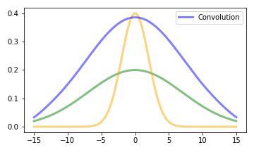
A convolution can be imagined as a weighting of one function with another. One of the functions is mirrored in the definition area and then pushed ‘piece by piece’ (infinitissimally small pieces!) over the other. The result is again a function that returns the ‘superposition’ of the two functions for each possible shift. If one imagines the convolution of two Gaussians, one can guess that the result must be a Gaussian funvtion (with slightly differed shape) again.

In the following i will show three different ways to solve the convolution mathematically.

Convolution in Time Domain

$$ \newcommand{\abs}[1]{\left\vert#1\right\vert} \newcommand{\br}[1]{\left ( #1 \right )} $$

Let’s assume two very simple Gaussians:

$$ \begin{eqnarray} f_1(t) &=& e^{-\br{\frac{t}{\sigma}}^2} \newline f_2(t) &=& e^{-\br{\frac{t}{r}}^2} \newline (f_1 * f_2)(t) &=& \int_{\mathbb{R}} f_1(t-\tau) \cdot f_2(\tau) ~d\tau \newline &=& \int_{\mathbb{R}} e^{-\br{\frac{t-\tau}{\sigma}}^2} \cdot e^{-\br{\frac{\tau}{r}}^2} ~d\tau \newline \end{eqnarray} $$

At this point you could try to do a partial integration. However, it makes more sense to separate the exponents of the e-functions in such a way that one obtains an e-function whose exponent is independent of the integration constant and can therefore be drawn in front of the integral.

$$ \begin{eqnarray} (f_1 * f_2)(t) &=& \int_{\mathbb{R}} e^{-\br{\br{\frac{t-\tau}{\sigma}}^2 + \br{\frac{\tau}{r}}^2}} ~d\tau \newline -\br{\br{\frac{t-\tau}{\sigma}}^2 + \br{\frac{\tau}{r}}^2}&=& -\frac{1}{\br{\sigma r}^2} \br{\sigma^2\tau^2 + r^2(t-\tau)^2} \newline &=& \frac{1}{\br{\sigma r}^2} \br{-\sigma^2\tau^2 - r^2 t^2 + r^2 2t\tau - r^2 \tau^2} \newline \text{(Square Addition)} &=& \frac{1}{\br{\sigma r}^2} \br{-r^2 t^2 + \frac{r^4 t^2}{r^2 + \sigma^2} - \frac{r^4 t^2}{r^2 + \sigma^2} + r^2 2t\tau - \br{r^2+\sigma^2} \tau^2} \newline &=& \frac{1}{\br{\sigma r}^2} \br{-r^2 t^2 + \frac{r^4 t^2}{r^2 + \sigma^2} -\br{r^2+\sigma^2} \br{r^4 t^2 - \frac{r^2 2t\tau}{r^2+\sigma^2} + \tau^2}} \newline &=& \frac{1}{\br{\sigma r}^2} \br{-\frac{r^2\sigma^2t^2}{r^2+\sigma^2} - \br{r^2+\sigma^2} \br{\tau-\frac{r^2 t}{r^2+\sigma^2}}^2} \newline &=& -\frac{t^2}{r^2+\sigma^2} - \frac{\br{r^2+\sigma^2}}{\br{r\sigma}^2} \br{\tau-\frac{r^2 t}{r^2+\sigma^2}}^2 \end{eqnarray} $$

$$ \begin{eqnarray} \Rightarrow (f_1 * f_2)(t) &=& \int_{\mathbb{R}} e^{-\frac{t^2}{r^2+\sigma^2} - \frac{\br{r^2+\sigma^2}}{\br{r\sigma}^2}\br{\tau-\frac{r^2 t}{r^2+\sigma^2}}^2} ~d\tau \newline &=& e^{-\frac{t^2}{r^2+\sigma^2}} \int_{\mathbb{R}} e^{-\frac{\br{r^2+\sigma^2}}{\br{r\sigma}^2}\br{\tau-\frac{r^2 t}{r^2+\sigma^2}}^2} ~d\tau \newline \end{eqnarray} $$

Now you have to know the following relationship in order to be able to solve the improper integral:

$$ \begin{eqnarray} \int_{\mathbb{R}} a\cdot e^{-bx^2} ~dx &=& a\cdot \sqrt{\frac{\pi}{b}} \end{eqnarray} $$

$$ \begin{eqnarray} \Rightarrow (f_1 * f_2)(t) &=& e^{-\frac{t^2}{r^2 + \sigma^2}} \cdot \sqrt{\frac{(r\sigma)^2\pi}{r^2 + \sigma^2}} \end{eqnarray} $$

The convolution of two Gaussians results in a scaled Gaussian. We guessed it already. The variance of the concolution is the sum of the variances of the two convoluted.

In general, the following applies (for the convolution of normal distributions):

$$ \begin{eqnarray} \mathcal{N}(\mu_1, \sigma_1) * \mathcal{N}(\mu_2, \sigma_2) &=& \mathcal{N}(\mu_1 + \mu_2, \sqrt{\sigma_1 + \sigma_2}) \end{eqnarray} $$

Fourier-Transformation of the Gaussians

$$ \begin{eqnarray} \mathcal{F} {f_1(t)} &=& \int_{\mathbb{R}} f_1(t) \cdot e^{-i\omega t} ~dt \newline &=& \int_{\mathbb{R}} e^{-\br{\frac{t}{\sigma}}^2} \cdot e^{-i\omega t} ~dt \newline &=& \int_{\mathbb{R}} e^{-\br{\frac{t^2}{\sigma^2} + i\omega t}} ~dt \end{eqnarray} $$

The exponent can be transformed using a square addition.

$$ \begin{eqnarray} \frac{1}{\sigma^2}(t+b)^2 &=& \frac{1}{\sigma^2}(t^2 + 2tb + b^2) \newline &=& \frac{1}{\sigma^2} t^2 + \frac{1}{\sigma^2} 2tb + \frac{1}{\sigma^2} b^2 \end{eqnarray} $$

A comparison of coefficients then shows that

$$ \begin{eqnarray} \frac{1}{\sigma^2} 2tb &=& i\omega t \newline \Leftrightarrow \frac{1}{\sigma^2} 2b &=& i\omega \newline \Rightarrow b &=& \frac{i\omega \sigma^2}{2} \end{eqnarray} $$

The exponent can thus be expressed as follows:

$$ \begin{eqnarray} \frac{1}{\sigma^2} \br{t + \frac{i\omega \sigma^2}{2}}^2 - \br{\frac{i\omega \sigma^2}{2}}^2 \end{eqnarray} $$

So you get

$$ \begin{eqnarray} \mathcal{F} {f_1(t)} &=& \int_{\mathbb{R}} e^{-\br{\frac{1}{\sigma^2} \br{t + \frac{i\omega \sigma^2}{2}}^2 - \br{\frac{i\omega \sigma^2}{2}}^2}} ~dt \newline &=& e^{\br{\frac{i\omega \sigma^2}{2}}^2} \cdot \int_{\mathbb{R}} e^{-\frac{1}{\sigma^2} \br{t + \frac{i\omega \sigma^2}{2}}^2} ~dt \newline \end{eqnarray} $$

When you know that

$$ \begin{eqnarray} \int_{\mathbb{R}} a\cdot e^{-bx^2} ~dx &=& a\cdot \sqrt{\frac{\pi}{b}} \end{eqnarray} $$

You can substitute the exponent ($x = \br{t + \frac{i\omega \sigma^2}{2}}^2$, $b=\frac{1}{\sigma^2}$) and receives

$$ \begin{eqnarray} \mathcal{F} {f_1(t)} &=& \sqrt{\sigma^2\pi} \cdot e^{\br{\frac{i\omega \sigma^2}{2}}^2} \newline \end{eqnarray} $$

One can see here that the Fourier transform of a Gaussian is also a Gaussian. The same applies to the inverse Fourier transformation.

Convolute by multiplying the Fourier-Transformations

A convolution in the time domain corresponds to a multiplication in the frequency domain and vice versa. Since the exponents add up when e-functions are multiplied and the coefficients also multiply, multiplying two Gaussianss also results in a Gaussian. Since the inverse Fourier transform of a Gaussian is also a Gaussian, the convolution of two Gaussians must also result in a Gaussian again.

Comments