In this post i’m giong to showing you how obtain the fourier coefficients of the complex fourier series for sawtooth and square waves. The approximation done by the fourier series (with a finite number of coefficients) is then compared to the original signal using a python script.

Sawtooth waves

The coefficients can be obtained this way:

$$ \begin{eqnarray} c_k &=& \frac{1}{T} \int_0^T f(t) \cdot e^{-j2 \pi k \frac{t}{T}} ~ dt \newline f(t) &=& t ~~~~\text{for $0 < t \le T$} \end{eqnarray} $$

By partial integration and correct substitution, we can solve the integral.

$$ \begin{eqnarray} u &=& t, ~ u’ = 1 \newline v’ &=& e^{-j2 \pi k \frac{t}{T}}, ~ v = \frac{-T}{j2 \pi k} \cdot e^{-j2 \pi k \frac{t}{T}}
\end{eqnarray} $$

$$ \begin{eqnarray} c_k &=& \left[ t \cdot \frac{-T}{j2 \pi k}e^{-j2 \pi k\frac{t}{T}} \right]^T_0 - \int^T_0 \frac{-1}{j2 \pi k} e^{-j2 \pi kt} ~ dt \newline &=& \frac{-T^2}{j2 \pi k} e^{-j2 \pi k} + \frac{1}{j2 \pi k} \int^T_0 e^{-j2 \pi kt} ~ dt \newline &=& \frac{-T^2}{j2 \pi k} + \left(\frac{1}{j2 \pi k}\right)^2 \left[ e^{-j2 \pi kt} \right]^T_0 \newline &=& \frac{-T^2}{j2 \pi k} + \left(\frac{1}{j2 \pi k}\right)^2 \left( e^{-j2 \pi kT} - 1 \right) \end{eqnarray} $$

If $T \in \mathbb{Z}$, the e-function will always become $1$. And thus the second part of the sum has to become $0$.

So if we choose $T$ to be $1$:

$$ \begin{eqnarray} c_1 , c_2 , …, c_n &=& \frac{-1}{j2 \pi k} \newline c_0 = \frac{1}{1} \int^1_0 t ~ dt &=& \frac{1}{2} \end{eqnarray} $$

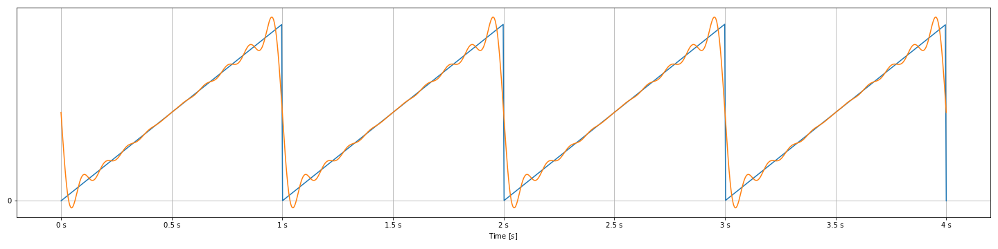
Thus the sawtooth can be described as follows.

$$ \begin{eqnarray} &\Rightarrow& f(t) = \frac{1}{2} + \sum_{k \in \mathbb{Z}, k \neq 0}\frac{j}{2 \pi k} e^{j2 \pi kt} \end{eqnarray} $$

import numpy as np
import matplotlib.pyplot as plt
import matplotlib.ticker as tck
from scipy import signal

time = np.linspace(0, 4, int(1e3))

# Time Period
T = 1
# The actual saw tooth wave
saw_wave = (signal.sawtooth(2 * np.pi * 1/T * time) + 1)/2

# Calc the complex fourier coefficients
def ck(k):
    if k == 0:
        return 1/2
    else:
        return -1 / (1j*2*np.pi*k)

def f(t, K):
    f = np.array([ck(k) * np.exp(1j*2*np.pi*k*t) for k in range(-K, K)])
    return f.sum()

# Number of coefficients to use.
# Because of range(-K,K) we will actually get n*2+1 coefficients
n = 10
fourier_series = np.array([f(t, n).real for t in time])
       
fig, ax = plt.subplots(1, 1, figsize=(20,5))

ax.set_xlabel('Time $[s]$ ')
ax.xaxis.set_major_formatter(tck.FormatStrFormatter('%g s'))
ax.yaxis.set_major_locator(tck.MultipleLocator(base=4))
ax.plot(time, saw_wave)
ax.plot(time, fourier_series)
ax.grid()

fig.tight_layout()
fig.savefig('fourier_series_saw.png')

Square waves

Periodicity by Convolution

Non periodical signals can be mathematically expressed preiodically by convoluting them with a series of Dirac delta functions. We will use this for the square wave to get the actual wave from a single sqaure.

$$ \newcommand{\brackets}[1]{\left ( #1 \right )} $$ $$ \begin{eqnarray} x(t) &=& \sum_{k\in\mathbb{Z}} x_0(t) \ast \delta(t-kt) \end{eqnarray}$$ $$ $$

By foruier transforming this now periodical function, one can reshape it in a way that it becomes easy to extract the fourier coefficients of the complex fourier series.

$$ \begin{eqnarray} \text{Complex Fourier Series: } x(t) &=& \sum_{k\in\mathbb{Z}} c_k \cdot e^{j2 \pi n \frac{t}{T}} \end{eqnarray} $$

$$ \begin{eqnarray} x(t) ~ \xrightarrow{\mathscr{F}} ~ X(f) &=& X_0(f) \cdot \frac{1}{T} \cdot \sum_{k\in\mathbb{Z}} \delta (f - \frac{k}{T}) \newline &=& \sum_{k\in\mathbb{Z}} \underbrace{\frac{1}{T} \cdot X_0(\frac{k}{T})}_{= c_k} \cdot \delta (f - \frac{k}{T}) \end{eqnarray} $$

$X_0(f)$ is the fourier transformation of the original function $x_0(t)$, which now represents the base period of the periodical function.

Fourier Series of the Square Wave

$$ \begin{eqnarray} rect\brackets{t} = \begin{cases} 1 & \text{if} ~|t| < 1 \newline \frac{1}{2} & \text{if} ~|t| = 1 \newline 0 & \text{if} ~|t| > 1 \end{cases} \label{eq_rect} \end{eqnarray} $$

The fourier transformation of a square looks like this:

$$ \begin{eqnarray} rect(t) ~ &\xrightarrow{\mathscr{F}}& ~ 2 si(\omega) \newline &=& 2 \frac{sin(\omega)}{\omega} \newline rect(\frac{t}{T}) ~ &\xrightarrow{\mathscr{F}}& ~ 2T si(\omega T) \newline &=& 2T \frac{sin(2\pi fT)}{2\pi fT} \newline &=& \frac{sin(2\pi fT)}{\pi f} \end{eqnarray} $$

$$ \begin{eqnarray} \text{Base Function:} \quad x_0(t) &=& \alpha \cdot rect(\frac{t}{T’}) \newline x(t) ~ \xrightarrow{\mathscr{F}} ~ X(f) &=& \alpha 2T’ \cdot si(\omega T’) \cdot \frac{1}{T} \sum_{k\in\mathbb{Z}} \delta(f-\frac{k}{T}) \newline &=& \alpha \frac{2T’}{T} \cdot si(2 \pi f T’) \cdot \sum_{k\in\mathbb{Z}} \delta(f-\frac{k}{T}) \newline &=& \sum_{k\in\mathbb{Z}} \alpha \frac{2T’}{T} \cdot si(2\pi \frac{T’}{T} k) \cdot \delta(f-\frac{k}{T}) \newline \end{eqnarray} $$

$$ \begin{eqnarray} \Rightarrow c_k &=& \alpha \frac{2T’}{T} \cdot si(2\pi \frac{T’}{T} k) \newline &=& \alpha \frac{2T’}{T} \cdot \frac{sin(2\pi \frac{T’}{T} k)}{2\pi \frac{T’}{T} k} \newline &=& \frac{\alpha}{\pi} \cdot \frac{sin(2\pi \frac{T’}{T} k)}{k} \end{eqnarray} $$

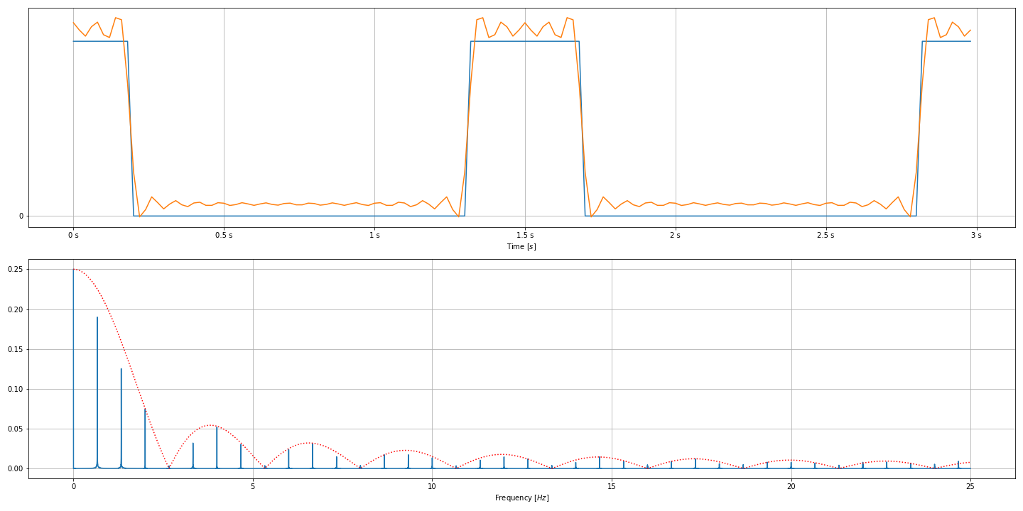
This image was created using the python script below. It shows a periodic sqaure wave, it’s frequency spectrum, the envelope of it’s spectrum ($si()$ the fourier transfomration of a singe square) and the reconstruction of the square wave with the complex fourier series using only 20 coefficients.

import numpy as np
import matplotlib.pyplot as plt
import matplotlib.ticker as tck
from scipy.fft import fft, fftfreq
from scipy import signal

f_max = 25 # in Hz
Ts = 1/(2 * f_max)

# Signal length [s]
sl = 1000

# Total number of samples
N = int(sl / Ts)

time = np.linspace(0, sl, N)

# Amplitude of the square wave
a = 1
# Time period of the square wave [s]
Tp = 1.5
# Width of the square [s]
Tw = Tp/4
# Shift the sqaure wave up, left, scale it to 1 and set the proper duty cycle
square_wave = a * (signal.square(2*np.pi/Tp*(time+Tw/2), duty=(Tw/Tp)) + 1) / 2

# Why do i need to do this?
# Did i get something wrong with the definition of the sqaure?
Tw = Tw/2

# Calc the complex fourier coefficients
def ck(k):
    if k == 0:
        # si(0) = 1
        return a / np.pi
    else:
        return a / np.pi * np.sin(2*np.pi*Tw/Tp*k) / (k)

def f(t, K):
    # We need coefficients positive 'k's only
    f = np.array([ck(k) * np.exp(1j*2*np.pi*k*t/Tp) for k in range(1, K+1)])
    return f.sum()

# Number of coefficients to use
n = 20
fourier_series = np.array([f(t, n).real for t in time])
# Why is this not scaling correctly?
# Because we are only calculating the upper HALF of the coefficients!
fourier_series *= 2
# The DC-part is somehow scaling correctly...
# Of course. It is the coefficiant sitting on the coordinate origin (point of symmetry)
fourier_series += ck(0)

# Frequency spectrum
yf0 = fft(square_wave)
# Scale it correctly
yf0 /= N

# Frequency axis values
xf = fftfreq(N, Ts)

# Fourier transformation of a rect is a sinc()
w =  2 * np.pi * xf
yf1 = a * 2*Tw/Tp * np.sin(w*Tw)/(w*Tw)
       
fig, ax = plt.subplots(2, 1, figsize=(20,10))

ax[0].set_xlabel('Time $[s]$ ')
ax[0].xaxis.set_major_formatter(tck.FormatStrFormatter('%g s'))
ax[0].yaxis.set_major_locator(tck.MultipleLocator(base=4))
# Plotting only the first second (visually nicer)
ax[0].plot(time[:int(3/Ts)], square_wave[:int(3/Ts)])
ax[0].plot(time[:int(3/Ts)], fourier_series[:int(3/Ts)])
ax[0].grid()

ax[1].set_xlabel('Frequency $[Hz]$')
# Plotting only the upper half of the freq-domain
# Be careful with the y-axis scaling!
ax[1].plot(xf[:N//2], np.abs(yf0[:N//2]))
ax[1].plot(xf[:N//2], np.abs(yf1[:N//2]), linestyle='dotted', color='red')
ax[1].grid()

fig.tight_layout()
fig.savefig('fourier_series_rect.png')

Comments